Individual Neural Tuning Model on simulated data

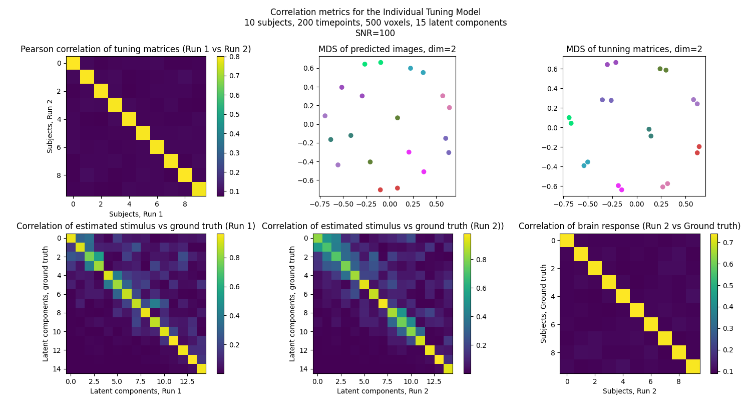
This is a toy experiment to test Individual Tuning Model (INT) on two parts of the data (or different runs) to assess the validity of tuning computation. This code has no intention to be an explanatory example, but rather a test to check the validity of the INT model.

To run this example, you must launch IPython via ipython --matplotlib in a terminal, or use jupyter-notebook.

import matplotlib.pyplot as plt
import numpy as np

from fmralign.alignment_methods import IndividualizedNeuralTuning as INT
from fmralign.fetch_example_data import generate_dummy_signal
from fmralign.hyperalignment.correlation import (
    compute_pearson_corr,
    matrix_MDS,
    stimulus_correlation,
    tuning_correlation,
)

Generate the data

In this example we use toy data to test the INT model. We generate two runs of the experiment, and we use the INT model to align the two runs. We then compare the tuning matrices and the shared response to assess the validity of the INT model. We also compare the reconstructed images to the ground truth to assess the validity of the INT model. The toy generation function allows us to get the ground truth stimulus and tuning matrices that were used to generate the data, and we can also control the level of noise in the data.

n_subjects = 10
n_timepoints = 200
n_voxels = 500
S_std = 5  # Standard deviation of the source components
T_std = 1
SNR = 100  # Signal to noise ratio
latent_dim = 15  # if None, latent_dim = n_t
decomposition_method = "pca"  # if None, SVD is used


(
    data_run_1,
    data_run_2,
    stimulus_run_1,
    stimulus_run_2,
    data_tuning,
) = generate_dummy_signal(
    n_subjects=n_subjects,
    n_timepoints=n_timepoints,
    n_voxels=n_voxels,
    S_std=S_std,
    T_std=T_std,
    latent_dim=latent_dim,
    SNR=SNR,
    seed=42,
)

parcels = [range(n_voxels)]

Create two independant instances of the model

We create two instances of the INT model to align the two runs of the experiment, then extract the tuning matrices and the shared from the two runs to compare them.

int1 = INT(
    n_components=latent_dim,
    parcels=parcels,
    decomp_method=decomposition_method,
)
int2 = INT(
    n_components=latent_dim,
    parcels=parcels,
    decomp_method=decomposition_method,
)
int1.fit(data_run_1, verbose=False)
int2.fit(data_run_2, verbose=False)

# save individual components
tuning_pred_run_1 = int1.tuning_data
tuning_pred_run_1 = np.array(tuning_pred_run_1)
tuning_pred_run_2 = int2.tuning_data
tuning_pred_run_2 = np.array(tuning_pred_run_2)

stimulus_pred_run_1 = int1.shared_response
stimulus_pred_run_2 = int2.shared_response

data_pred = int1.transform(data_run_2)

Predict : stimulus matrix shape:  (200, 15)

Plotting validation metrics

We compare the tuning matrices and the shared response to assess the validity of the INT model. To achieve that, we use Pearson correlation between true and estimated stimulus, as well as between true and estimated tuning matrices. For tuning matrices, this is dones by first computing the correlation between every pair of tuning matrices from the two runs of the experiment, and then averaging the correlation across the diagonal (ie the correlation between the same timepoint of the two runs).

fig, ax = plt.subplots(2, 3, figsize=(15, 8))


# Tunning matrices
correlation_tuning = tuning_correlation(tuning_pred_run_1, tuning_pred_run_2)
ax[0, 0].imshow(correlation_tuning)
ax[0, 0].set_title("Pearson correlation of tuning matrices (Run 1 vs Run 2)")
ax[0, 0].set_xlabel("Subjects, Run 1")
ax[0, 0].set_ylabel("Subjects, Run 2")
fig.colorbar(ax[0, 0].imshow(correlation_tuning), ax=ax[0, 0])

random_colors = np.random.rand(n_subjects, 3)
# MDS of predicted images
corr_tunning = compute_pearson_corr(data_pred, data_run_2)
data_pred_reduced, data_test_reduced = matrix_MDS(
    data_pred, data_run_2, n_components=2, dissimilarity=1 - corr_tunning
)

ax[0, 1].scatter(
    data_pred_reduced[:, 0],
    data_pred_reduced[:, 1],
    label="Run 1",
    c=random_colors,
)
ax[0, 1].scatter(
    data_test_reduced[:, 0],
    data_test_reduced[:, 1],
    label="Run 2",
    c=random_colors,
)
ax[0, 1].set_title("MDS of predicted images, dim=2")

# MDS of tunning matrices
corr_tunning = compute_pearson_corr(tuning_pred_run_1, tuning_pred_run_2)
T_first_part_transformed, T_second_part_transformed = matrix_MDS(
    tuning_pred_run_1,
    tuning_pred_run_2,
    n_components=2,
    dissimilarity=(1 - corr_tunning),
)

ax[0, 2].scatter(
    T_first_part_transformed[:, 0],
    T_first_part_transformed[:, 1],
    label="Run 1",
    c=random_colors,
)
ax[0, 2].scatter(
    T_second_part_transformed[:, 0],
    T_second_part_transformed[:, 1],
    label="Run 2",
    c=random_colors,
)
ax[0, 2].set_title("MDS of tunning matrices, dim=2")
# Set square aspect
ax[0, 1].set_aspect("equal", "box")
ax[0, 2].set_aspect("equal", "box")

# Stimulus matrix correlation
correlation_stimulus_true_est_first_part = stimulus_correlation(
    stimulus_pred_run_1.T, stimulus_run_1.T
)
ax[1, 0].imshow(correlation_stimulus_true_est_first_part)
ax[1, 0].set_title("Correlation of estimated stimulus vs ground truth (Run 1)")
ax[1, 0].set_xlabel("Latent components, Run 1")
ax[1, 0].set_ylabel("Latent components, ground truth")
fig.colorbar(
    ax[1, 0].imshow(correlation_stimulus_true_est_first_part), ax=ax[1, 0]
)

correlation_stimulus_true_est_second_part = stimulus_correlation(
    stimulus_pred_run_2.T, stimulus_run_2.T
)
ax[1, 1].imshow(correlation_stimulus_true_est_second_part)
ax[1, 1].set_title(
    "Correlation of estimated stimulus vs ground truth (Run 2))"
)
ax[1, 1].set_xlabel("Latent components, Run 2")
ax[1, 1].set_ylabel("Latent components, ground truth")
fig.colorbar(
    ax[1, 1].imshow(correlation_stimulus_true_est_second_part), ax=ax[1, 1]
)


# Reconstruction
corr_reconstruction = tuning_correlation(data_pred, data_run_2)
ax[1, 2].imshow(corr_reconstruction)
ax[1, 2].set_title("Correlation of brain response (Run 2 vs Ground truth)")
ax[1, 2].set_xlabel("Subjects, Run 2")
ax[1, 2].set_ylabel("Subjects, Ground truth")
fig.colorbar(ax[1, 2].imshow(corr_reconstruction), ax=ax[1, 2])


plt.rc("font", size=10)
# Define small font for titles
fig.suptitle(
    "Correlation metrics for the Individual Tuning Model\n"
    + f"{n_subjects} subjects, {n_timepoints} timepoints, {n_voxels} voxels, {latent_dim} latent components\n"
    + f"SNR={SNR}"
)

plt.tight_layout()
plt.show()