2.2. Functional alignment pipeline

As seen in the previous section, functional alignment search for a transform between images of two or several subjects in order to match voxels which have similar profile of activation. This section explains how this transform is found in fmralign to make the process easy, efficient and scalable.

We compare various methods of alignment on a pairwise alignment problem for Individual Brain Charting subjects. For each subject, we have a lot of functional informations in the form of several task-based contrast per subject. We will just work here on a ROI.

2.2.1. Local functional alignment

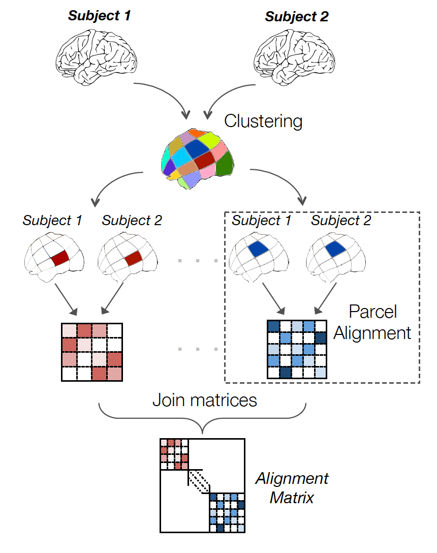
Aligning images of various size is not always easy because when we search a transformation for n voxels yields at least a complexity of \(n^2\). Moreover, finding just one transformation for similarity of functional signal in the whole brain could create unrealistic correspondances, for example inter-hemispheric.

To avoid these issues, we keep alignment local, i.e. on local and functionally meaningful regions. Thus, in a first step cluster the voxels in the image into n_pieces sub-regions, based on functional information. Then we find local alignment on each parcel and we recompose the global matrix from these.

With this technique, it is possible to find quickly sensible alignment even for full-brain images in 2mm resolution. The parcellation chosen can obviously have an impact. We recommend ‘ward’ to have spatially compact and reproducible clusters.

2.2.2. Alignment methods on a region

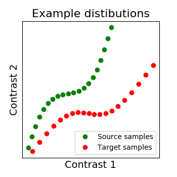
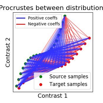
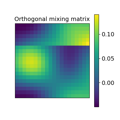
Full code example on 2D simulated data

All the figures in this section were generated from a dedicated example: Alignment on simulated 2D data.

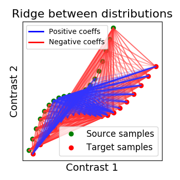
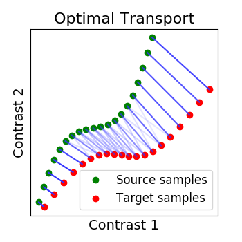
As we mentionned several times, we search for a transformation, let’s call it R, between the source subject data X and the target data Y. X and Y are arrays of dimensions (n_voxels, n_samples) where each image is a sample. So we can see each signal as a distribution where each voxel as a point in a multidimensional functional space (each dimension is a sample).

We show below a 2D example, with 2 distributions: X in green, Y in red. Both have 20 voxels (points) characterized by 2 samples (images). And the alignment we search for is the matching of both distibutions, optimally in some sense.

2.2.2.1. Orthogonal alignment (Procrustes)

The first idea proposed in Haxby, 2011 was to compute an orthogonal mixing matrix R and a scaling sc such that Frobenius norm \(||sc RX - Y||^2\) is minimized.

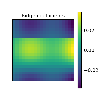
2.2.2.2. Ridge alignment

Another simple idea to regularize the transform R searched for is to penalize its L2 norm. This is a ridge regression, which means we search R such that Frobenius norm \(|| XR - Y ||^2 + alpha * ||R||^2\) is minimized with cross-validation.

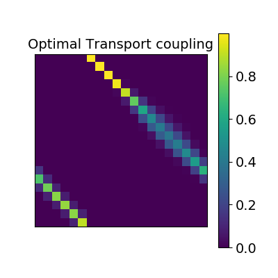
2.2.2.3. Optimal Transport alignment

Finally this package comes with a new method that build on the Wasserstein distance which is well-suited for this problem. This is the framework of Optimal Transport that search to transport all signal from X to Y while minimizign the overall cost of this transport. R is here the optimal coupling between X and Y with entropic regularization.

2.2.3. Comparing those methods on a region of interest

Full code example

The full code example of this section is : Alignment methods benchmark (pairwise ROI case).

Now let’s compare the performance of these various methods on our simple example: the prediction of left-out data for a new subject from another subjects data.

2.2.3.1. Loading the data

We begin with the retrieval of images from two Individual Brain Charting subjects :

>>> from fmralign.fetch_example_data import fetch_ibc_subjects_contrasts
>>> files, df, mask = fetch_ibc_subjects_contrasts(['sub-01', 'sub-02'])

Here files is the list of paths for each subject and df is a pandas Dataframe with metadata about each of them.

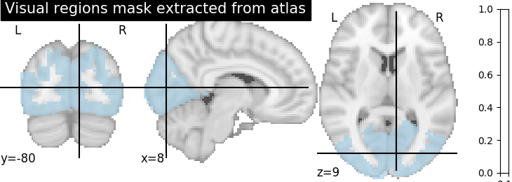
2.2.3.2. Extract a mask for the visual cortex from Yeo Atlas

>>> from nilearn import datasets, plotting
>>> from nilearn.image import resample_to_img, load_img, new_img_like
>>> atlas_yeo_2011 = datasets.fetch_atlas_yeo_2011()
>>> atlas = load_img(atlas_yeo_2011.thick_7)

Select visual cortex, create a mask and resample it to the right resolution

>>> mask_visual = new_img_like(atlas, atlas.get_data() == 1)
>>> resampled_mask_visual = resample_to_img(
    mask_visual, mask, interpolation="nearest")

Plot the mask we use

>>> plotting.plot_roi(resampled_mask_visual, title='Visual regions mask extracted from atlas',
         cut_coords=(8, -80, 9), colorbar=True, cmap='Paired')

2.2.3.3. Define a masker

>>> from nilearn.input_data import NiftiMasker
>>> roi_masker = NiftiMasker(mask_img=mask).fit()

2.2.3.4. Prepare the data

For each subject, for each task and conditions, our dataset contains two independent acquisitions, similar except for one acquisition parameter, the encoding phase used that was either Antero-Posterior (AP) or Postero-Anterior (PA). Although this induces small differences in the final data, we will take advantage of these “duplicates” to create a training and a testing set that contains roughly the same signals but acquired independently.

The training fold, used to learn alignment from source subject toward target:

• source train: AP contrasts for subject ‘sub-01’

• target train: AP contrasts for subject ‘sub-02’

>>> source_train = df[df.subject == 'sub-01'][df.acquisition == 'ap'].path.values
>>> target_train = df[df.subject == 'sub-02'][df.acquisition == 'ap'].path.values

The testing fold:

• source test: PA contrasts for subject ‘sub-01’, used to predict the corresponding contrasts of subject ‘sub-02’

• target test: PA contrasts for subject ‘sub-02’, used as a ground truth to score our predictions

>>> source_test = df[df.subject == 'sub-01'][df.acquisition == 'pa'].path.values
>>> target_test = df[df.subject == 'sub-02'][df.acquisition == 'pa'].path.values

2.2.3.5. Define the estimators, fit them and do a prediction

To proceed with alignment we use the class PairwiseAlignment with the masker we created before.

First we choose a suitable number of regions such that each regions is approximately 200 voxels wide.

>>> n_voxels = roi_masker.mask_img_.get_data().sum()
>>> n_pieces = np.round(n_voxels / 200)

Then for each method we define the estimator, fit it, and predict new image. We then plot the correlation of this prediction with the real signal. We also include identity (no alignment) as a baseline.

>>> from fmralign.pairwise_alignment import PairwiseAlignment
>>> from fmralign._utils import voxelwise_correlation
>>> methods = ['identity','scaled_orthogonal', 'ridge_cv', 'optimal_transport']

>>> for method in methods:
>>>   alignment_estimator = PairwiseAlignment(alignment_method=method, n_pieces=n_pieces, mask=roi_masker)
>>>   alignment_estimator.fit(source_train, target_train)
>>>   target_pred = alignment_estimator.transform(source_test)
>>>   aligned_score = voxelwise_correlation(target_test, target_pred, roi_masker)
>>>   display = plotting.plot_stat_map(aligned_score, display_mode="z", cut_coords=[-15, -5],
>>>         vmax=1, title=f"Correlation of prediction after {method} alignment")

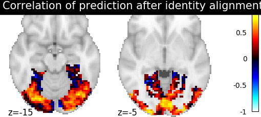
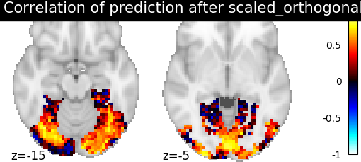
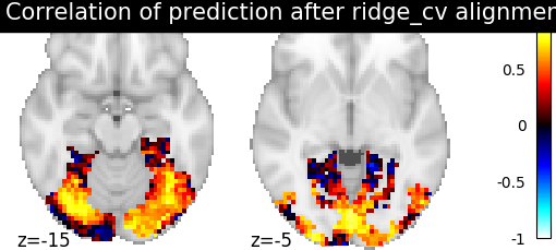
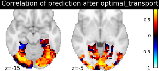
We can observe that all alignment methods perform better than identity (no alignment). Ridge is the best performing method, followed by Optimal Transport. If you use Ridge though, be careful about the smooth predictions it yields.